Assessing the robustness of HOI using bootstrap

The bootstrap method involves repeatedly resampling the dataset with replacement to simulate multiple datasets. By analyzing these resampled datasets, one can gain insights into the variability of statistics, such as mean, variance, or in this case, the significance of multiplets. This technique is particularly useful when the underlying distribution is complex or unknown. In this project, the primary goal is to identify the multiplets that have a substantial impact on the dataset based on statistical significance. The bootstrap approach will provide a more robust way of identifying these multiplets compared to traditional methods. Additionally, confidence interval estimation will be integrated into the process, allowing for a better understanding of the range of possible values for the multiplet significance.
Published on July 01, 2023 by Dishie Vinchhi
bootsrap confidence intervals resampling
- Resampling the Input Data
To perform bootstrapping, we need to resample the input data. This involves randomly sampling data points from the original dataset with replacement. Each resampled dataset should have the same length as the original dataset and values can be repeated within.
- Selecting Significant Multiplets
Once we have resampled datasets, we can compute the desired metric, o-information on each resampled dataset. This step allows us to evaluate the metric’s value on different subsets of the original data.
- Compute Confidence Intervals
With the resampled metric values, we can estimate confidence intervals to quantify the uncertainty associated with the metric. One common approach is to calculate the percentiles of the resampled metric values. For example, computing the 5th and 95th percentiles will give a 90% confidence interval. These percentiles represent the lower and upper bounds of the confidence interval, respectively.
Code for bootci
Step-by-step explanation of the code
- Generating all possible combinations of given size of multiplets
for msize in range(minsize, maxsize + 1):
    # generate combinations
    n_features=x.shape[1]
    combs = combinations(n_features+1, msize)
- Resampling input x for each combination nboot times
eg. x = [1,2,3]
resampled_x = [1, 2 ,1] , [3, 3, 1] , etc
for i in range(n_boots):
      part = resample(x.T, n_samples=x.shape[2], random_state=0 + i).T ## reshaping of x : make correction (transpose)
- Calculate the oinfo using the resampled part for each combination and keep appending the value of oinfo to a list
      # copnorm and demean the resampled partition
      part = copnorm_nd(part.copy(), axis=0)
      part = part - part.mean(axis=0, keepdims=True)

      # make the data (n_variables, n_features, n_trials)
      part = jnp.asarray(part.transpose(2, 1, 0))

      # calcualte oinfo
      # print(part.shape)
      _, _oinfo = jax.lax.scan(oinfo_mmult,part, combs)

      flattened_list = list(itertools.chain.from_iterable(np.asarray(_oinfo)))
      val.extend(flattened_list)
- Calculating the 5th and 95th percentile of the oinfo and plotting the results.
    ci = np.stack(val,axis=0)
    # oinfo values within [0.05, 0.95] of bounds
    p5 = np.nanpercentile(ci, 5, axis=0)
    p95 = np.nanpercentile(ci, 95, axis=0)
    filtered_data = [x for x in ci if p5 <= x <= p95]
    final.extend(filtered_data)
  # Plotting the histogram
  plt.hist(final, bins=20, color='C2', alpha=.2)
  plt.xlabel('oinfo')
  plt.ylabel('Frequency')
  plt.title('Histogram')

  # Marking the 25th and 75th percentile
  plt.axvline(np.nanpercentile(final, 25), color='k', lw=2, ls='--')
  plt.axvline(np.nanpercentile(final, 75), color='k', lw=2, ls='--')
  return p5, p95
Complete code as a function bootci
def bootci(x, n_boots):
  minsize = 3
  maxsize=5
  oinfo,ci=[],[]
  final = []
  val=[]
  for msize in range(minsize, maxsize + 1):
    n_features=x.shape[1]
    combs = combinations(n_features+1, msize)
    for i in range(n_boots):
      part = resample(x.T, n_samples=x.shape[2], random_state=0 + i).T ## reshaping of x : make correction (transpose)

      part = copnorm_nd(part.copy(), axis=0)
      part = part - part.mean(axis=0, keepdims=True)

      part = jnp.asarray(part.transpose(2, 1, 0))

      _, _oinfo = jax.lax.scan(oinfo_mmult,part, combs)
      flattened_list = list(itertools.chain.from_iterable(np.asarray(_oinfo)))
      val.extend(flattened_list)

    ci = np.stack(val,axis=0)
    p5 = np.nanpercentile(ci, 5, axis=0)
    p95 = np.nanpercentile(ci, 95, axis=0)
    filtered_data = [x for x in ci if p5 <= x <= p95]
    final.extend(filtered_data)

  # Plotting the histogram
  plt.hist(final, bins=20, color='C2', alpha=.2)
  plt.xlabel('oinfo')
  plt.ylabel('Frequency')
  plt.title('Histogram')
  plt.axvline(np.nanpercentile(final, 25), color='k', lw=2, ls='--')
  plt.axvline(np.nanpercentile(final, 75), color='k', lw=2, ls='--')
  return p5, p95
Confidence Interval Plotted by the function
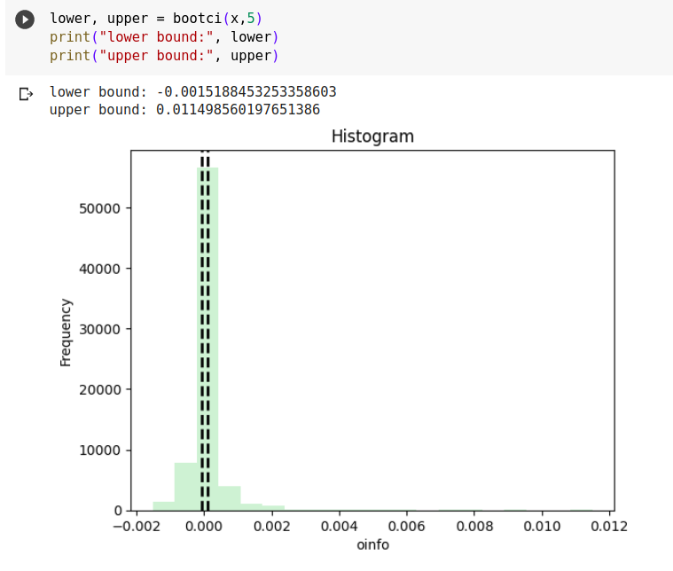
Here, the number of times a particular oinfo value occurs (frequency of oinfo) is plotted against the oinfo. The black dotted plots are the p5 (5th percentile) and p95 (95th percentile) of the values of oinfo. These give a 90% confidence interval of the oinfo range.